Benchmark: lateral viscosity
What validates the 3-D path today. The 3-D viscosity path is cross-checked against two things only: VILMA1, on the last deglaciation (deglaciation page), and the low-viscosity-zone case of Weerdesteijn et al. (2023) (Weerdesteijn et al. 2023) (LVZ page). No multi-code 3-D benchmark has been run yet. This page describes the setup that VILMA2 contributes to such a benchmark. It produces the protocol files and compares them with nothing.
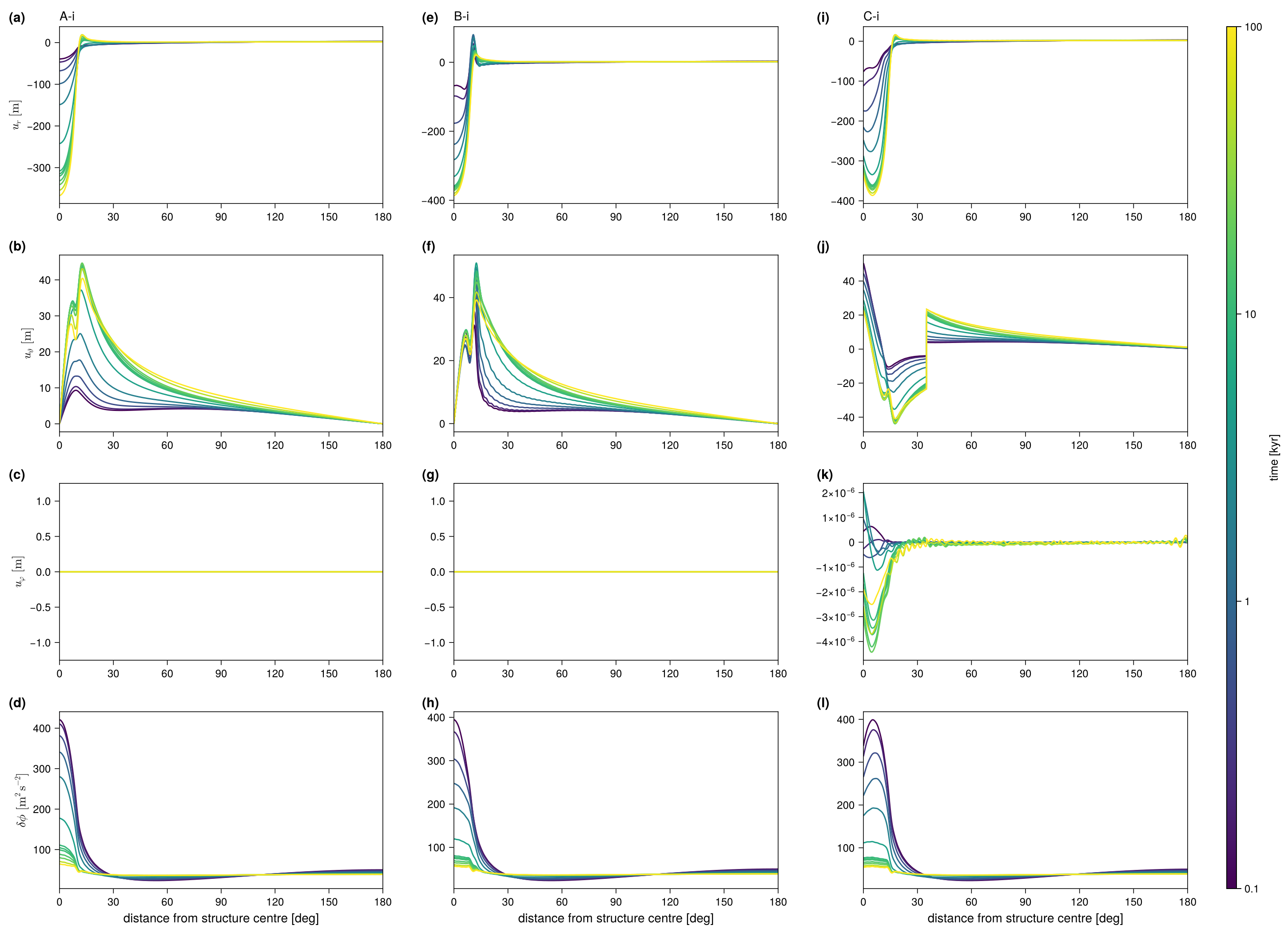
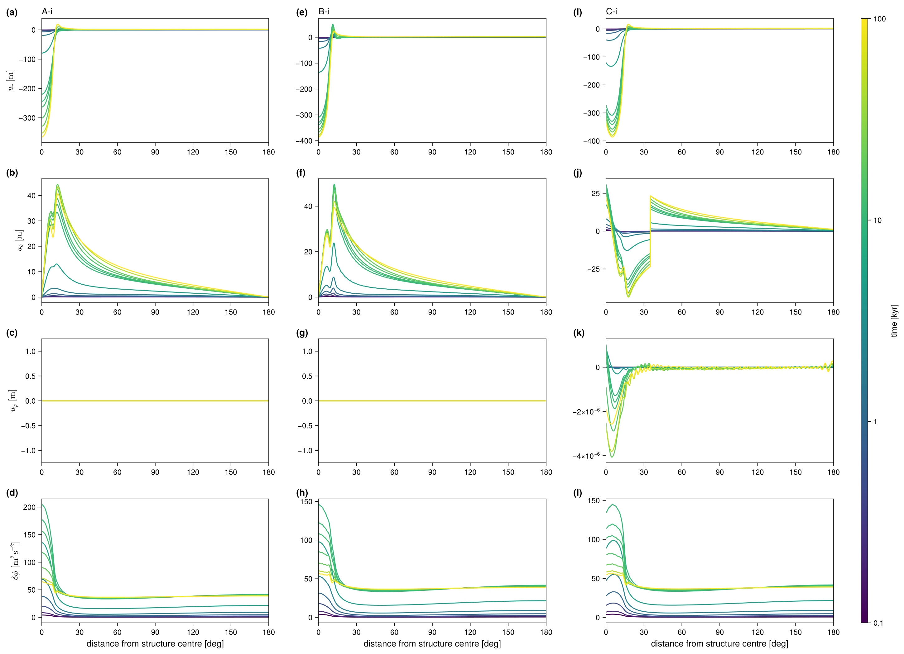
The benchmark follows Spada et al. (2011) and Martinec et al. (2018) but adds a low-viscosity column under or near an ice load. It isolates the effect of lateral viscosity on vertical and horizontal displacement, on the gravitational potential, and on geocentre motion. The note defines compressible and incompressible variants; VILMA2 is incompressible, so only A-i, B-i and C-i are run.
Setup
Earth. M3–L70–V01 (as for the Love numbers), with interfaces added at 60 and 220 km depth so that FE nodes bound the structure. The 60–70 km part of the lithosphere is made Maxwell with \(\eta = 10^{30}\) Pa s, because an elastic element cannot carry a lateral viscosity. This split changes the test-A result by \(\lesssim 4\times10^{-9}\) relative.
Structure. A rotationally symmetric column over 60–220 km depth, centred at \((\vartheta_S, \lambda_S)\), with a smoothed-Heaviside profile in the angular distance \(\vartheta\) from its centre:
\[ \log_{10}\eta = \log_{10}\eta_\text{ref} + \left(\log_{10}\eta_c - \log_{10}\eta_\text{ref}\right) H(\vartheta), \qquad H(\vartheta) = \left[1 + e^{2(\vartheta-\vartheta_w)/d}\right]^{-1}, \]
with half-width \(\vartheta_w = 12°\), edge width \(d = 1°\) and centre viscosity \(\eta_c = 10^{18}\) Pa s. That is a drop of 3 orders of magnitude in the mantle and 12 in the 60–70 km lithosphere, which the note asks to reach the same centre value.
Grid. The Gauss grid has \(2\ell_\max + 2\) latitudes. It has \(4\ell_\max\) longitudes for C and 2 for the axisymmetric A and B.
Load. A cap of radius \(\alpha = 10°\) with a square-root profile,
\[ \sigma(\vartheta) = \rho_\text{ice}\, h_L \sqrt{\frac{\cos\vartheta - \cos\alpha}{1 - \cos\alpha}}, \qquad h_L = 1500\ \mathrm{m},\ \rho_\text{ice} = 931\ \mathrm{kg\,m^{-3}}, \]
centred at \((\vartheta_L, \lambda_L)\). Its SH coefficients are exact: Gauss–Legendre quadrature in \(s\) with \(\cos\vartheta = \cos\alpha + (1-\cos\alpha)s^2\) turns the square-root edge into a polynomial, and the addition theorem rotates the cap to its centre. Two forcings: heav (load applied at \(t=0\)) and ramp (thickness linear over 0–10 kyr, then held). No ocean, no rotation.
| test | structure \((\vartheta_S, \lambda_S)\) | load \((\vartheta_L, \lambda_L)\) | geometry |
|---|---|---|---|
| A-i | none (S0) | (0°, 0°) | 1-D reference |
| B-i | (0°, 0°) | (0°, 0°) | axisymmetric, structure under load |
| C-i | (35°, 25°) | (30°, 25°) | off-axis, structure and load overlap |
A and B are axisymmetric and run with \(m_\max = 0\); C runs the full spectrum.
Time stepping. Explicit (fe) memory update. \(\Delta t\) is set by the Maxwell ceiling at \(\eta_c\) (\(\mu\Delta t/\eta_c \le 1\)), rounded to divide 100 yr, which gives \(\Delta t = 0.448\) yr. All three tests use the same \(\Delta t\), so their differences come from the structure alone.
Readings of the setup note
The note is a draft and a few points had to be interpreted:
- The half-width of the structure is 12° in the text and 10° in the table; 12° is used.
- \(\Delta\eta = -10^3\) is read as a factor \(10^{-3}\) in log space (the formula in the note gives \(\eta = 0\) for S0, \(\Delta\eta = 0\)).
- The prose swaps the ice and water densities; the table’s values (\(\rho_\text{ice} = 931\), \(\rho_w = 1000\)) are used.
- “\(\vartheta_S\) and \(\alpha\) are increased” in the ramp is read as the Spada et al. (2011) ramp: the ice thickness grows linearly, the geometry is fixed.
- The model’s own constants (seconds per year, \(G\)) are used; they differ from the note’s by \(\lesssim 10^{-4}\) relative.
Output
At the epochs 0.1, 0.2, 0.5, 1, 2, 5, 10, 11, 12, 15, 20, 50 and 100 kyr, the fields are evaluated at points every 0.1°. The points lie along the great circle from the structure centre through the load centre to the antipode. For A and B, where both centres sit at the pole, that circle is the \(\lambda = 0\) meridian. The files follow the protocol (tab-delimited, # header):
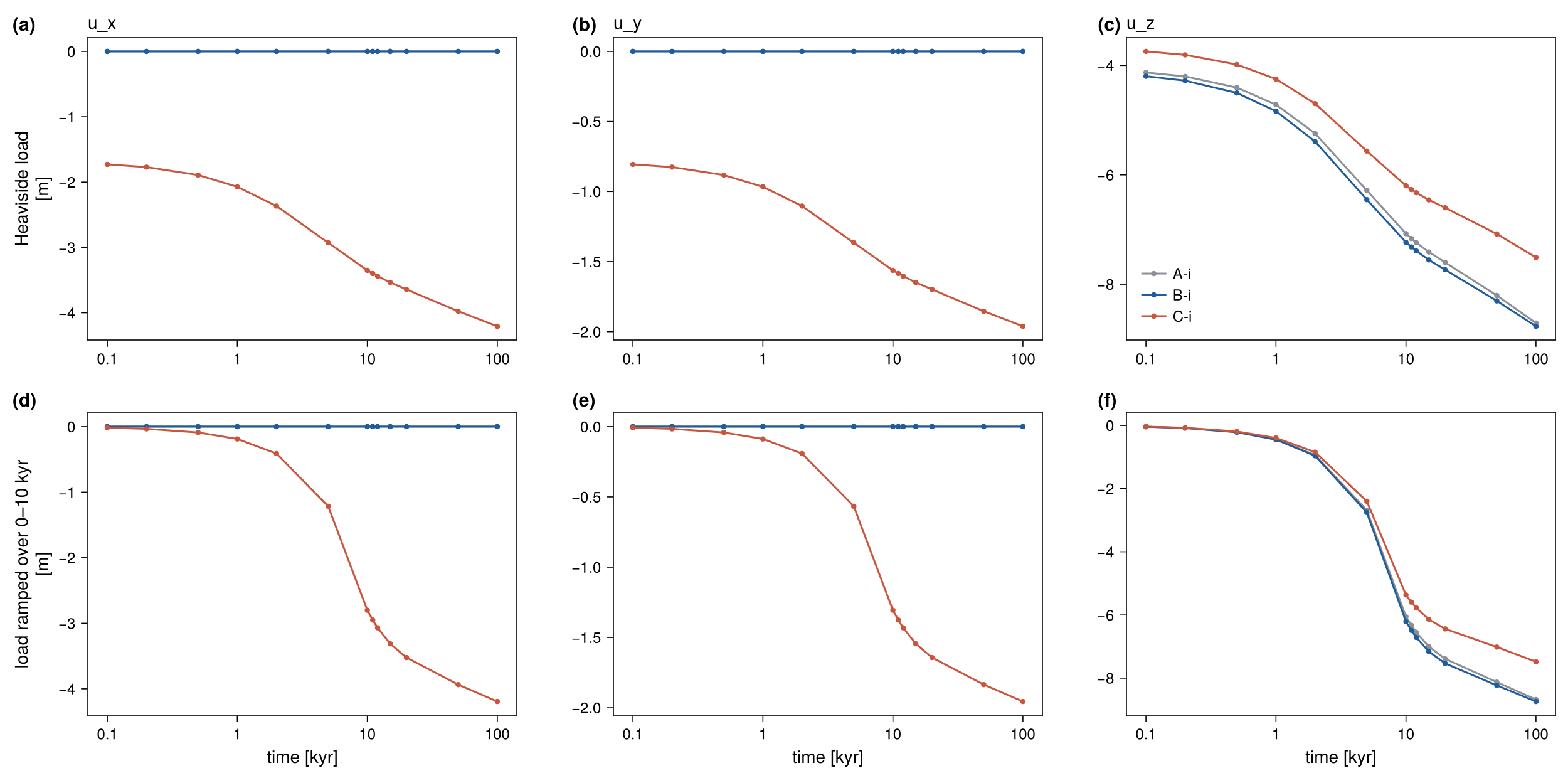
disp_VILMA2_<T>-i_<forcing>.txt: longitude, latitude, distance along the section [deg], time [kyr], \(u_r\), \(u_\vartheta\), \(u_\varphi\) [m] and \(\delta\phi\) [m² s⁻²].gcm_VILMA2_<T>-i_<forcing>.txt: time [kyr] and the geocentre offset \(u_\text{gcm} = u_\text{CF} - u_\text{CM}\) (\(x, y, z\) [m]).
The driver does not compare these files with a reference, and it returns no pass or fail. The only check it prints is the load mass, from the degree-0 coefficient, next to its closed form. It also prints \(u_r\) at the structure centre at each output epoch.
Conventions:
- Frame. Displacements are in the CM frame (
deg1_frame = "cm"). Then \(u_\text{gcm} = u_\text{CF}\), the surface mean of the displacement vector, \((U_1 + 2V_1)/3\) in Cartesian components (Blewitt 2003). - Potential. \(\delta\phi = -F(a) = g N\), which includes the load’s own potential.
- Horizontal displacement is spheroidal plus toroidal. Its components are in the local geographic basis, so \(u_\vartheta\) changes sign where the section crosses a pole. At the pole itself, the basis is that of the meridian the section runs along.
Running
The run config is examples/bench_visc3d.nml. Its &benchv3d group sets test (A/B/C), forcing (heav/ramp) and time_end [years]. From &vilma only lmax, l_toroidal and visc_3d_tol are read. The example config sets lmax = 128 and l_toroidal = .true., and visc_3d_tol keeps its default. The earth model, memory scheme, degree-1 frame and grid are fixed by the benchmark. The protocol files are written to the working directory.
Build, then submit all six cases as one runme ensemble (runme alias visc3d):
make bench_visc3d openmp=1
runme -o runs/bench_visc3d -e visc3d -n examples/bench_visc3d.nml --omp 64 \
      -p benchv3d.test=A,B,C benchv3d.forcing=heav,ramp -s
Use -r instead of -s to run locally, and add e.g. vilma.lmax=64 benchv3d.time_end=2000 for a short test. The validation suite runs the benchmark as its stage B and draws the figures and tables on this page (validation/README.md):
cd validation
./run.sh B                          # A-i, B-i, C-i, both forcings, l_max 128
LMAX=64 CASES="A B" ./run.sh B      # truncation series; also LMAX=256
./run.sh submit reduce analyse      # tables/blockB.md and the figures
Restart. A run longer than one job is split into segments. restart_out saves the memory state at time_end, and restart_in resumes from it. Time is counted in global steps, so a chain of segments reproduces one uninterrupted run byte for byte. Each segment appends to the protocol files and skips the epochs already written. A restart from another test, forcing, \(\ell_\max\) or \(\Delta t\) is refused. For 20-kyr segments:
&benchv3d  test = "C"  forcing = "heav"  time_end = 40.0e3
           restart_in = "restart_20kyr.nc"  restart_out = "restart_40kyr.nc" /
The step count is set by \(\eta_c\): 223 000 steps to 100 kyr. At \(\ell_\max = 64\) with 8 threads (laptop), a C run costs about 53 ms per step, or about 3.3 h. A and B, with \(m_\max = 0\), take minutes. The target resolution is \(\ell_\max = 128\), where C takes about 20 h on 64 threads. That is why C runs in restart segments.
Result
All six cases (A-i, B-i, C-i, each with heav and ramp forcing) have been run to 100 kyr at \(\ell_\max = 128\) with the toroidal field on, as five 20-kyr restart segments each. A and B were also run at \(\ell_\max = 64\) and 256. The load mass matches the closed form exactly. The numbers are from validation/tables/blockB.md (model f0c4678, albedo) and equal those of the earlier model 907bc74 to the printed digits.
| test | forcing | \(u_r\) at load, 0.1 kyr | 10 kyr | 100 kyr | max \(u_r\) at 100 kyr | \(\lvert u_\text{gcm}\rvert\) at 100 kyr |
|---|---|---|---|---|---|---|
| A-i | heav | \(-39.35\) m | \(-307.76\) m | \(-366.67\) m | 17.90 m | 8.709 m |
| B-i | heav | \(-67.91\) m | \(-357.80\) m | \(-386.07\) m | 20.76 m | 8.769 m |
| C-i | heav | \(-67.11\) m | \(-360.55\) m | \(-386.46\) m | 15.40 m | 8.829 m |
| A-i | ramp | \(-0.36\) m | \(-219.71\) m | \(-365.64\) m | 18.02 m | 8.676 m |
| B-i | ramp | \(-0.55\) m | \(-309.13\) m | \(-385.60\) m | 21.02 m | 8.739 m |
| C-i | ramp | \(-0.53\) m | \(-308.11\) m | \(-386.02\) m | 15.49 m | 8.797 m |
The low-viscosity column under the load (B-i) deepens the depression at 0.1 kyr by about 70 % and at 100 kyr by about 5 %. These numbers have no reference yet.
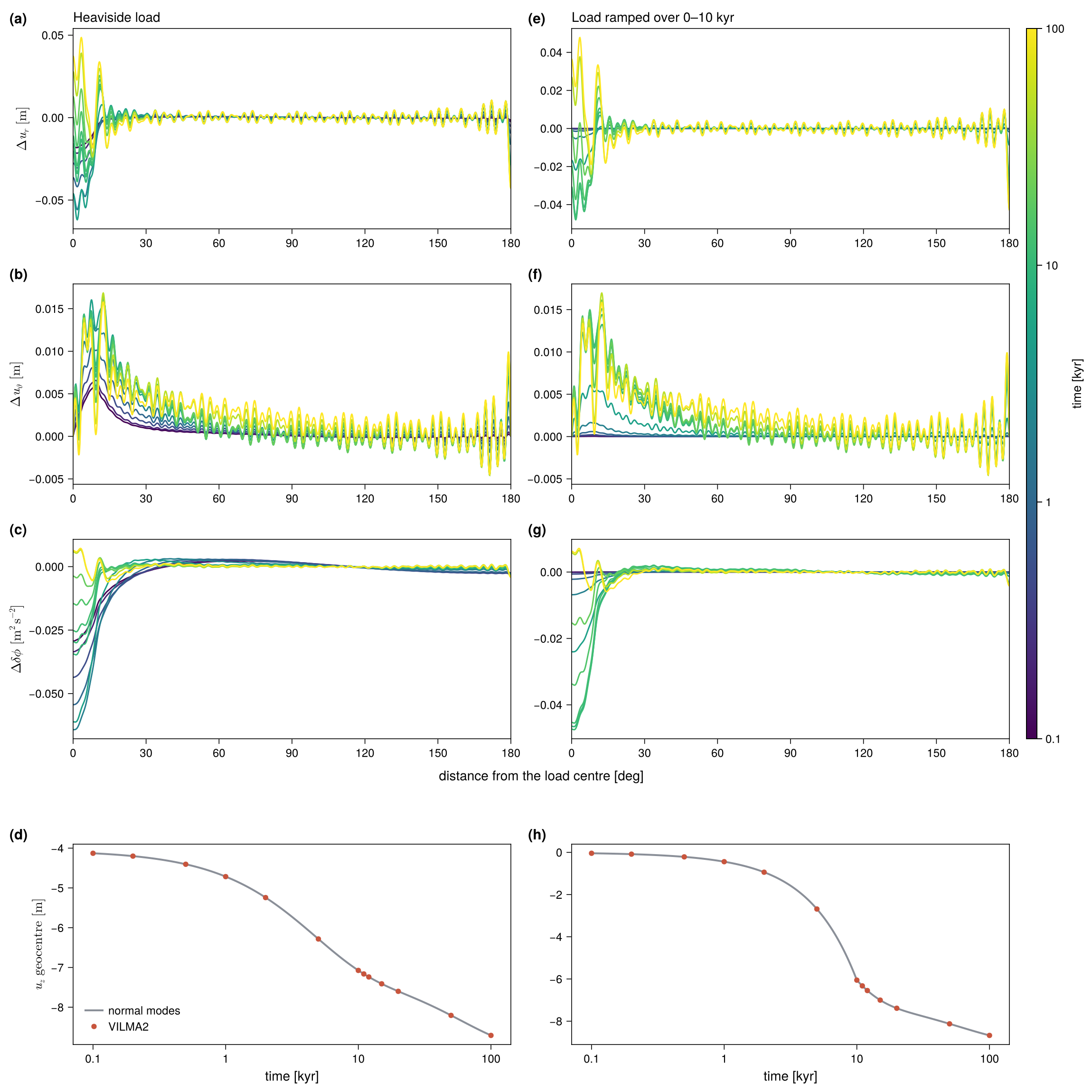
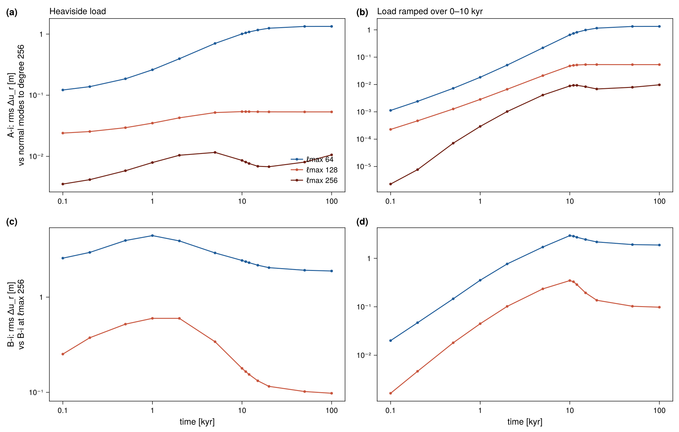
Test A-i against an exact solution. A-i has no lateral structure, so its exact solution is the normal-mode response of M3–L70–V01 at the same truncation. VILMA2 matches it to within 0.05 m in \(u_r\) (of 39–367 m at the load center), 0.016 m in \(u_\vartheta\) and 1.6 mm in the geocentre offset, at 0.1, 1, 10 and 100 kyr and for both forcings.
Truncation. The rms difference of \(u_r\) along the section between A-i and the normal-mode solution to degree 256 is 1.3 m at \(\ell_\max = 64\), 0.05 m at 128 and 0.01 m at 256 (100 kyr, heav). For B-i against its own \(\ell_\max = 256\) run it is 1.9 m at 64 and 0.1 m at 128. At \(\ell_\max = 64\) the 1° edge of the structure is not resolved and B-i shows Gibbs ringing with a period of about 3°.
Cost. At \(\ell_\max = 128\) with the toroidal field on and 64 threads (albedo), C-i took 19.3 h (heav) and 20.0 h (ramp) to 100 kyr, 3.5–4.2 h per 20-kyr segment. A-i and B-i, with \(m_\max = 0\), took 0.07 h and 0.16 h. On levante (model 907bc74), C-i took 10.5 h with the toroidal field off and 18.6 h with it on, so the toroidal field costs a factor of 1.8.
Figures
The figures show VILMA2 only. A comparison with other codes follows once their results are available.