Benchmark: the sea-level equation

Reference: Martinec et al. (2018), the SLE intercomparison (Martinec et al. 2018), cases A and C2/D3/E2/F1 (SBK reference curves). Tests: test_benchmark_martinec (case A, in make check) and test_benchmark_sle (the four SLE cases, in make check-slow). Asserted: case A within 1.5 % (uplift, horizontal) and 3 % (geoid) of the profile peak; SLE cases within 30 % (uplift), 35 % (horizontal), 12 % (geoid), 8 % (sea surface) and 12 % (relative sea level) of the profile peak. Measured (ifx, albedo): case A 0.5–1.9 %; cases D3, E2 and F1 at most 7.6 %; case C2 up to 28 %, see below.

This benchmark runs the full self-consistent, migrating-coastline sea-level equation driven by the viscoelastic response. It is the benchmark in which VILMA1 took part. It exercises the ocean function, mass conservation, coastline migration, grounded-ice flotation, and the sub-grid sloping coast all together.

Benchmark structure

The authority for the case definitions is Martinec et al. (2018), Table 4 (not the differing case labels in third-party reimplementations). The paper defines five cases from a small set of building blocks:

Ice (square-root cap \(h(\psi) = h_0\sqrt{(\cos\psi-\cos\alpha)/(1-\cos\alpha)}\), \(\alpha=10°\)): L0 pole/1500 m; L1 colat 25°/lon 75°, 1500 m; L2 same centre, 500 m.
Basin (\(\zeta^{(0)} = b_{\max} - b_0\,e^{-\psi^2/2\sigma^2}\), \(\sigma=26°\)): B0 none; B1 colat 100°/lon 320°, shallow (760/1200); B2 colat 35°/lon 25°, deep (3800/6000, 2200 m at centre).
Time: T0 Heaviside (load held, \(t_f = 10\) kyr); T1 linear growth over 10 kyr then held to 15 kyr.
Ocean: SLE0 none; SLE1 fixed geometry \(O^{(0)}\); SLE2 time-varying (migrating coastline).
Densities \(\rho_{\text{ice}}/\rho_{\text{water}} = 931/1000\ \mathrm{kg\,m^{-3}}\), \(g_0 = 9.815\ \mathrm{m\,s^{-2}}\).

The vendored SBK reference files use a labelling offset by one letter from the paper (SBK letter = paper letter + 1):

SBK	paper	ocean	ice	time	basin
A	A	SLE0 (none)	L0 (1500 m)	T0	B0 (none)
C2	B	SLE1 fixed	L1 (1500 m)	T0	B1 (shallow)
D3	C	SLE1 fixed	L2 (500 m)	T1	B2 (deep)
E2	D	SLE2 migrate	L2 (500 m)	T1	B2 (deep)
F1	E	SLE2 migrate	L2 (500 m)	T1	B2* (paleo-topo prescribed)

Error measure

Every number on this page is a peak-normalized maximum error: the largest absolute difference between model and reference along one profile, divided by the largest absolute value of the reference along that same profile. The two horizontal components are normalized by the peak magnitude of the horizontal vector, since a profile through a symmetry axis nulls one component. This measure is strict in one respect and misleading in another. It reports the single worst point of a profile. It also grows without any change in the absolute error when a profile crosses a region where the field itself is small. Both effects appear in case C2.

Case A — pure viscoelastic loading

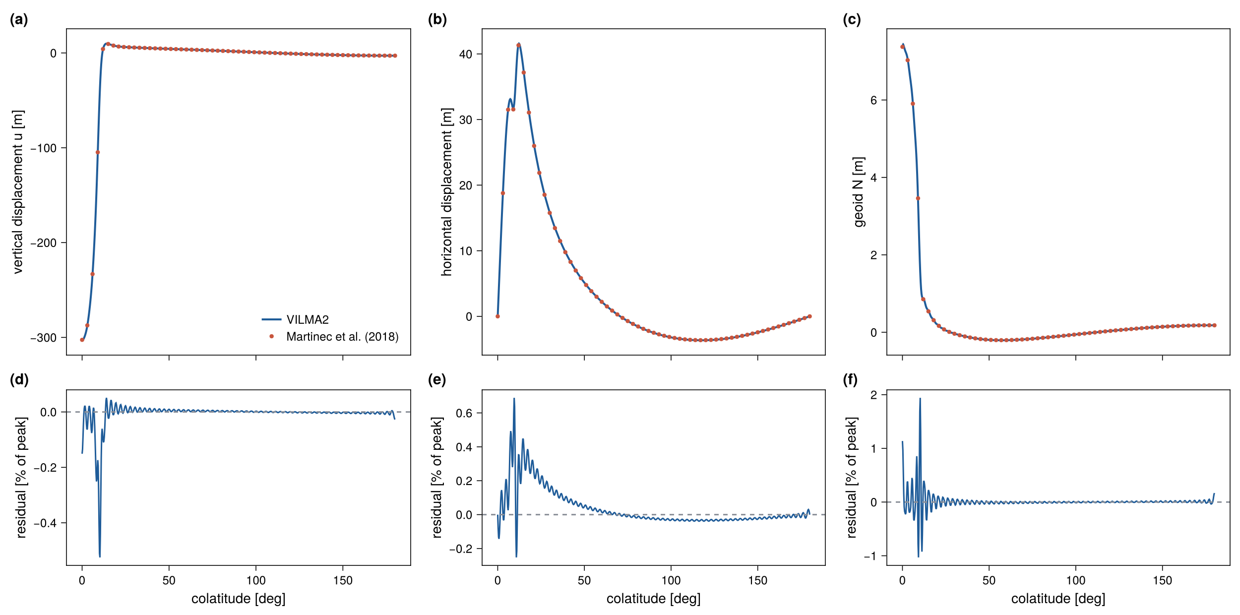
The simplest case is a spherical cap applied as a Heaviside load and relaxed for 10 kyr, with no ocean and with degrees 0 and 1 dropped. test_benchmark_martinec compares the profiles of fig. 10 of Martinec et al. (2018).

Table 1: Case A, model 1790f86, ifx, albedo.

Field	Peak	Tolerance	Measured
uplift	302.6 m	1.5 %	0.52 %
horizontal displacement	41.4 m	1.5 %	0.69 %
geoid	7.4 m	3 %	1.94 %

This is the first benchmark of the horizontal displacement and confirms the spheroidal \(V\) field.

Figure 1: Case A, 10 kyr after a 1500 m spherical cap (10° radius) is applied: (a) vertical displacement, (b) horizontal displacement and (c) geoid along colatitude, VILMA2 (line) and the reference of Martinec et al. (2018), fig. 10 (dots, every tenth point). (d–f) VILMA2 minus the reference, in percent of the profile’s peak. The oscillation near the cap edge is the truncation of the cap’s sharp edge at degree 128.

SLE cases — C2, D3, E2, F1

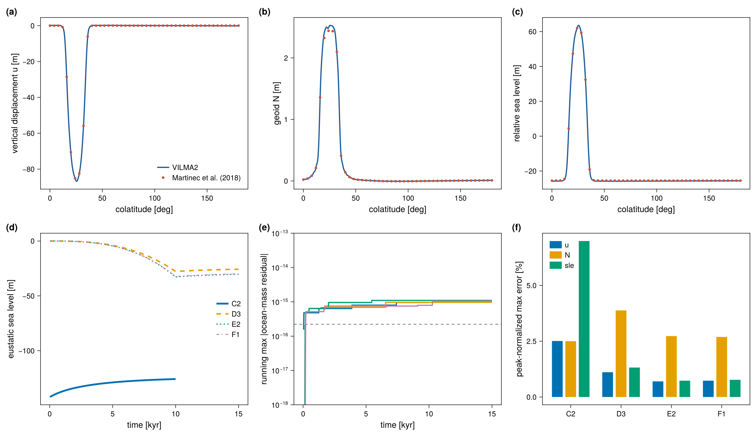
These cases run the full sea-level equation with the time-varying load at \(\ell_\max = 128\) with a 20 yr step. The reference files give seven columns: longitude or colatitude, vertical displacement, the two horizontal components, the gravitational potential increment, the sea-surface variation, and the SLE result (relative sea level). They are sampled along four profiles per case (figs. 10–13 of the paper). Figs. 10 and 11 pass through the ice cap, along a meridian and a parallel. Figs. 12 and 13 pass through the ocean basin.

Mass is conserved to \(\sim 10^{-16}\) (relative) per step in every case. Three settings control the agreement:

Fixed or migrating ocean. C2 and D3 are fixed-ocean (SLE1) cases. Running them with a migrating coastline drains the basin roughly twice too far, so the fixed-ocean mode (sle_fixed_ocean) must be honored.
Grounded-ice masking. The ice load applies only over grounded ice. Floating ice over the deep basin is carried by the ocean term.
The sub-grid sloping coast (sle_subgrid). The SBK reference uses a sub-grid coast. With a binary coastline the local errors of E2 near the grounding line were 14–42 % during development (not re-measured for this page; test_benchmark_sle.x E2 binary runs that variant). With the sub-grid water-column load they are about 1 %.

Measured errors

The table gives the peak-normalized maximum error [%] of every profile and field (model 1790f86, ifx, albedo, make check-slow).

Table 2: Peak-normalized maximum error [%] against the SBK reference curves.

Case	Profile	\(u\)	\(v_\theta\)	\(v_\varphi\)	\(N\)	sea surface	rsl
C2	fig. 10	2.51	14.29	9.12	2.50	4.96	6.99
C2	fig. 11	2.47	15.00	11.77	1.34	5.01	6.93
C2	fig. 12	23.10	27.73	7.20	7.16	4.95	7.16
C2	fig. 13	21.42	25.73	24.34	5.41	4.92	6.85
D3	fig. 10	1.11	1.64	6.04	3.88	0.92	1.32
D3	fig. 11	0.72	3.42	4.03	5.42	1.23	1.07
D3	fig. 12	5.12	4.73	5.04	5.33	0.89	1.70
D3	fig. 13	3.31	4.21	4.44	6.98	0.93	1.80
E2	fig. 10	0.70	3.86	7.57	2.73	0.92	0.73
E2	fig. 11	0.38	3.33	5.25	1.46	0.93	0.87
E2	fig. 12	5.00	5.02	4.93	4.79	0.93	1.30
E2	fig. 13	2.83	3.93	5.04	6.97	0.94	1.83
F1	fig. 10	0.73	3.56	7.02	2.69	0.88	0.77
F1	fig. 11	0.37	3.35	5.11	1.51	0.89	0.82
F1	fig. 12	6.38	4.92	4.93	5.28	0.87	1.42
F1	fig. 13	2.83	3.96	4.95	6.78	0.90	1.80
	tolerance	30	35	35	12	8	12

The final uniform sea-level shift of the model is \(-125.83\) m (C2), \(-25.74\) m (D3), \(-30.28\) m (E2) and \(-29.93\) m (F1).

What the numbers mean

Cases D3, E2 and F1. The sea surface and relative sea level agree with the reference to within 2 % of the peak in all twelve profiles, which is 0.2–0.8 m in absolute terms. The uplift through the ice cap agrees to about 1 % (0.4–1.0 m of 86–102 m). The percentages of 5–7.6 % belong to fields with a small peak along the profile: the uplift along the basin profiles (0.35–0.5 m of 7–15 m), the horizontal displacement (0.4–0.8 m of 7–15 m) and the geoid (0.02–0.14 m of 0.3–2.7 m). The absolute differences are thus below 1 m everywhere in these three cases.

Case C2. The differences are larger, and the percentages of 21–28 % are not a local effect at the migrating coastline (the ocean of C2 is fixed). Two smooth, large-scale differences explain them. First, the sea surface of the model lies 5.9 m below the reference at every point of all four profiles, which is 4.9 % of the 120 m sea-level fall of this case. Second, the uplift differs from the reference by a smooth pattern of global extent with an amplitude of about 7 m. It is positive on the side of the ice cap and negative on the far side, which is the shape of a degree-1 term. The absolute uplift difference is therefore about the same in all four profiles (7.3–7.8 m). It is 2.5 % of the 309 m peak along the profiles through the ice cap, and 21–23 % of the 34 m peak along the two profiles through the basin. The horizontal differences of 6–7 m behave in the same way. Case C2 has the thickest ice (1500 m, three times that of the other cases) applied as a Heaviside load on a fixed ocean, so a difference in the degree-0 and degree-1 treatment between the two codes is largest here. The same pattern is present in E2 with an amplitude of about 0.3 m. The origin of this difference (reference frame, or the mass budget of the fixed ocean) has not been attributed. The tolerances of the test (30 % and 35 %) are set to pass this case and are therefore not a meaningful bound for the other three.

An inter-code comparison, not an analytic one

The SBK reference is the output of one code (giapy), not a closed-form solution. Martinec et al. (2018) document a scatter of a few percent between the participating codes. The agreement of D3, E2 and F1 is within that scatter. The uniform offset and the degree-1 pattern of C2 are larger than that and remain open.

Figures

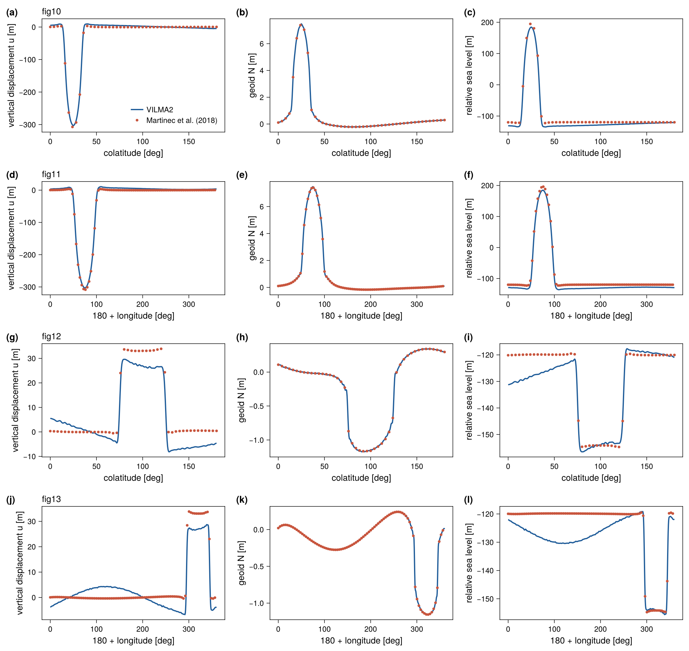
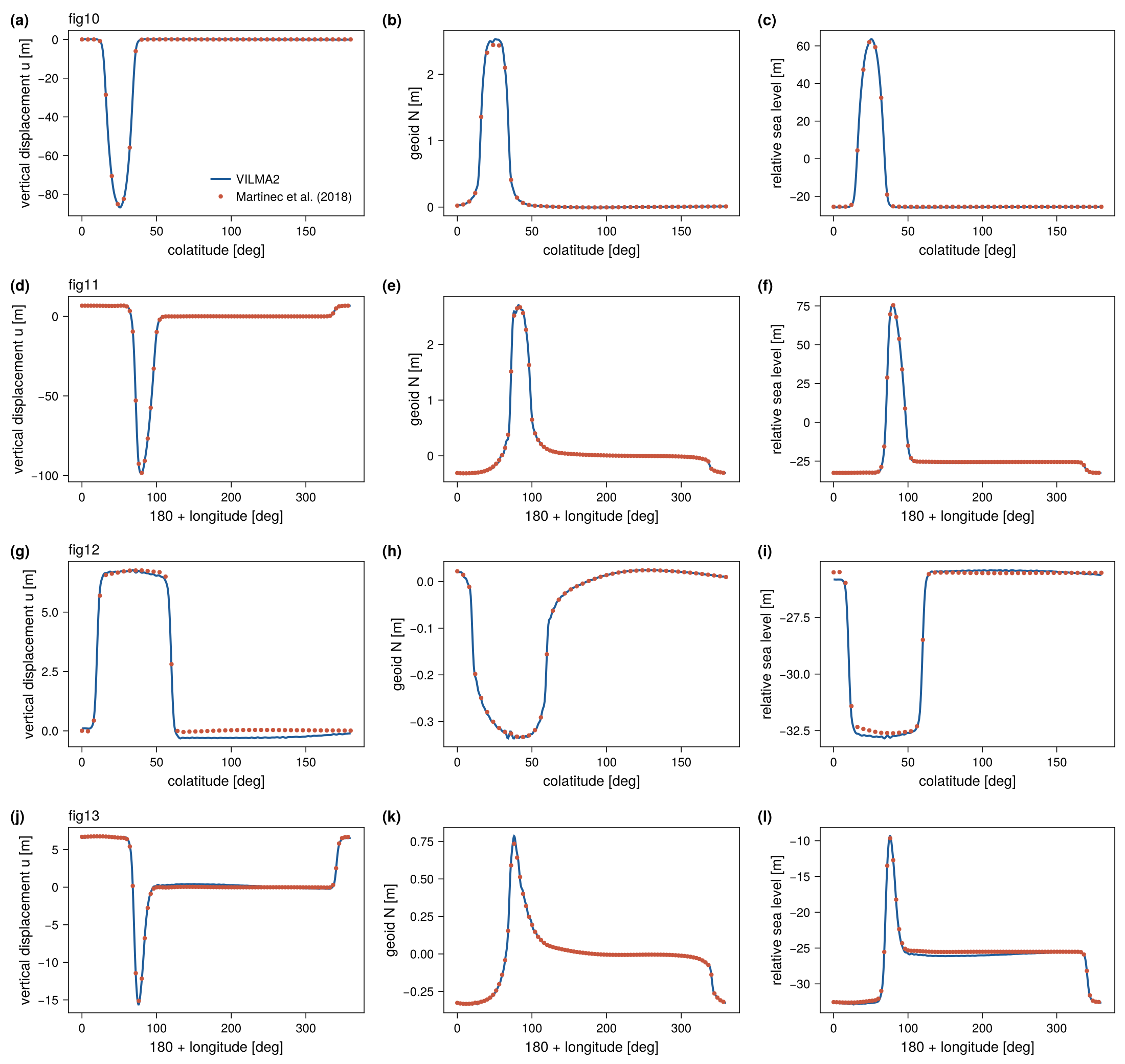
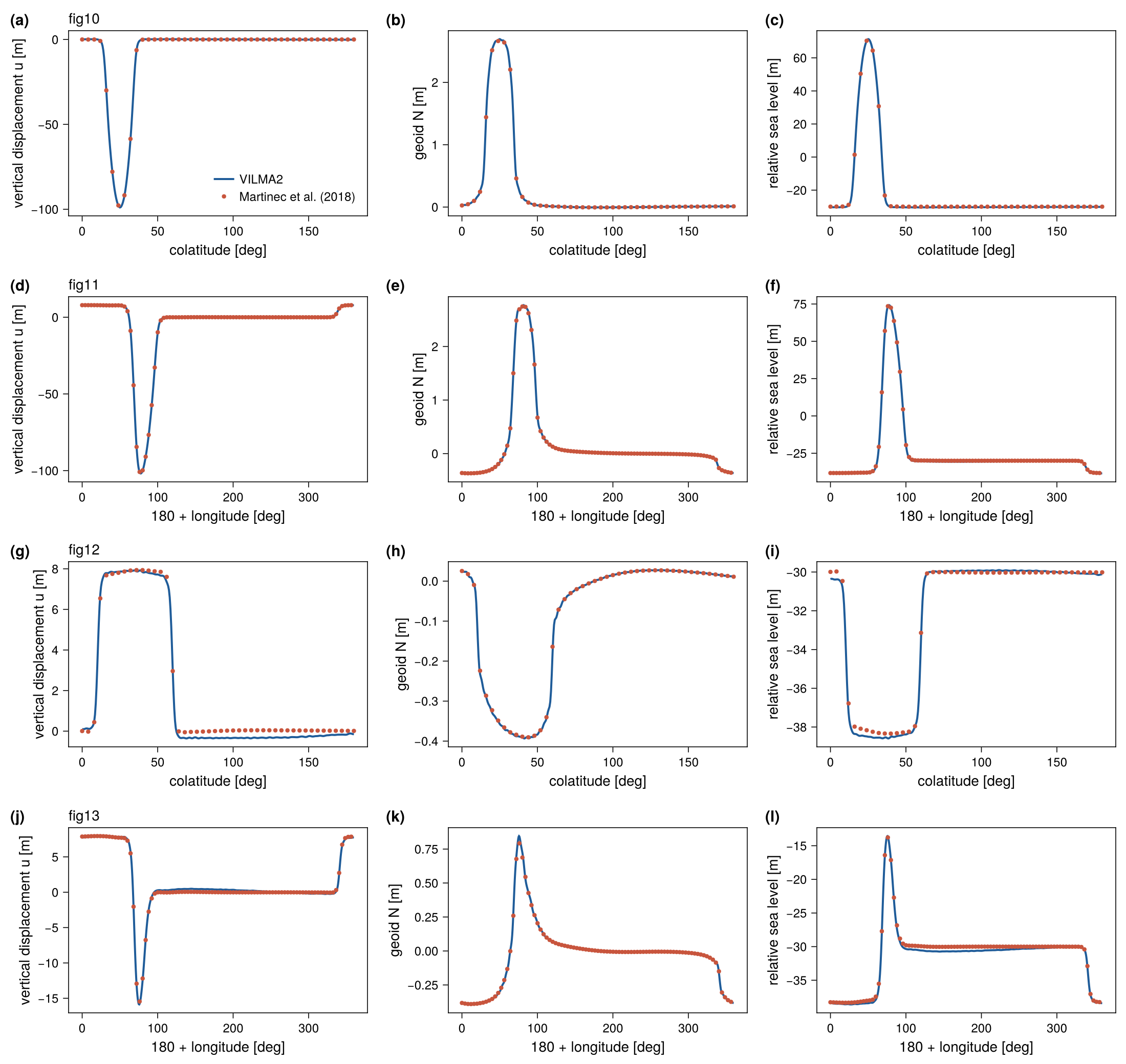
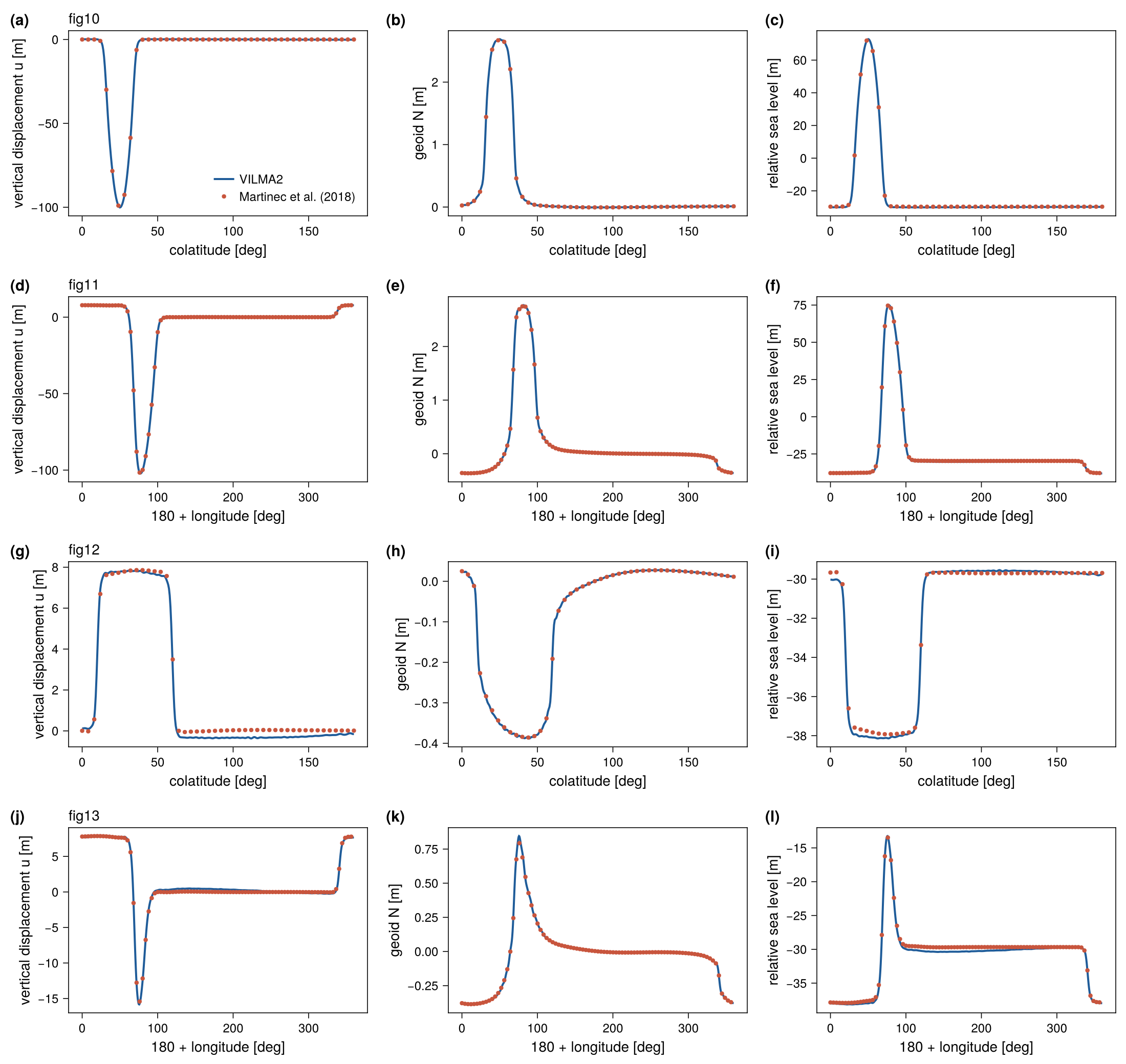
Figure 2: Summary of the SLE cases: (a–c) vertical displacement, geoid and relative sea level along one reference profile, VILMA2 and the reference of Martinec et al. (2018); (d) eustatic sea level against time for C2, D3, E2 and F1; (e) running maximum of the relative ocean-mass residual; (f) peak-normalized maximum error per field.

Figure 3: Case C2: profiles of uplift, horizontal displacement, geoid, sea surface and relative sea level along the four reference profiles (figs. 10–13), VILMA2 and the SBK reference.

With VILMA_BENCH_DUMP set, test_benchmark_sle writes the model and reference values of every profile (sle_<case>_<fig>_profile.txt) and the time history of each run (sle_<case>_history.txt); see Benchmarks.

Provenance

Reference: data/benchmarks/sle_martinec2018/*_SBK.dat, from the giapy package (tests/sbk_benchmark_data.tar.gz, MIT), originating in the Martinec et al. (2018) intercomparison. The case ↔︎ paper mapping and column definitions are in data/benchmarks/PROVENANCE.md.

References

Martinec, Z., V. Klemann, W. van der Wal, et al. 2018. “A Benchmark Study of Numerical Implementations of the Sea Level Equation in GIA Modelling.” Geophysical Journal International 215 (1): 389–414. https://doi.org/10.1093/gji/ggy280.