Deglaciation: VILMA1 versus VILMA2

Pre-publication page. This page is not linked from the navigation and is excluded from the site search. It is reachable by direct link only.

Reference: VILMA1 (Martinec 2000; Martinec et al. 2018), run through VILMA2’s own driver with solver = "v1". Earth structure: the 3-D viscosity field of Bagge et al. (2021) and its radial mean. Driver: vilma.x (not in make check; needs a VILMA1 install). Status: ✅ run at \(\ell_\max = 170\), model f0c4678, albedo; VILMA2’s 3-D run with the toroidal field on, the model default. The numbers below are from validation/tables/ of that pass.

This page compares VILMA2 with VILMA1 on the last deglaciation. Both solvers run behind the same driver, so they share the ice forcing, the remap, the reference state, the output grid and the output file layout. The comparison is a change of one namelist key, solver = "v2" or solver = "v1". It tests the complete model at production resolution: the visco-elastic response with 3-D viscosity, the sea-level equation with migrating coastlines, and the rotational feedback.

It is a code-to-code comparison, not a comparison with a reference solution. Agreement shows that the two codes solve the same problem in the same way. It does not bound the error that both codes share.

Experiment design

The settings below are common to both solvers unless stated. They are set in validation/experiments/nml/blockD.nml.tmpl and blockDV1.nml.tmpl.

item	setting
Ice forcing	GLAC-1D ice thickness, `input/geo_ice_glac1d_deglac.nc`, 26 ka to present, 261 slices every 100 yr
Ice density	931 kg m⁻³ (the value of the earlier reference results; the model default is 917)
Coupling and output grid	\(\ell_\max = 170\), Gauss grid of VILMA2
VILMA1 internal grid	`vilma_v1_jmax = 170`, 512 × 256
Reference state	`i_eq = 2`, VILMA2’s LGM reference state, the same file for both solvers
Viscosity, case 3-D	the field of Bagge et al. (2021) on longitude, latitude and radius, with VILMA2’s clamp applied (\(10^{19.5}\) to \(10^{30}\) Pa s)
Viscosity, case 1Db	the radial mean of that field (the geometric mean per level)
Degree-1 frame	center of mass in both (`deg1_frame = "cm"`)
Radial elastic structure	PREM geometry in 11 layers, VILMA2’s layer table, also given to VILMA1
Radial mesh	the 5/10/40 km element spacing of VEGA in both. VILMA2: 220 elements including the fluid core (`mesh_depth = 80e3, 670e3`), 82 of them 3-D. VILMA1: 128 mantle and lithosphere elements, from a `densi.inp` written from VILMA2’s layer table
Ice and water density	VILMA2’s values, also written to VILMA1’s load file
Rotation	on in both
Coastlines	migrating, with the subgrid (water-column) ocean load
VILMA2 time stepping	`scheme = "fe"`, equal sub-steps at the Maxwell stability limit within the 100 yr interval
VILMA1 time stepping	`vilma_v1_nsub = 12` uniform sub-steps of 8.33 yr
Toroidal field	VILMA2: on in the 3-D run (`l_toroidal = .true.`, the model default); a control run with it off measures its effect. The 1Db runs have no laterally 3-D element for it to act on

Reference state. The reference is built once, by VILMA2 with the 3-D viscosity. The 26 ka ice load is held for 30 kyr from rest (equil_time_max = 30000, equil_rate_tol = 0, no 1-D pre-spin-up, lid rule off). The result is not an equilibrium, because the stiffest parts of the viscosity field keep relaxing. The fixed duration makes the state reproducible. Both solvers start from this state, so the load anomaly is zero at the start for both. VILMA1 requires this: it starts with zero load anomaly and zero viscous memory. Neither solver runs a spin-up in the comparison itself (equil_time_max = 0, pre_spinup_1d = .false.).

Viscosity. VILMA1 reads its viscosity file directly and applies no clamp of its own. The file it reads is therefore written from VILMA2’s clamped field, on the 128 radial elements that VILMA1 uses. VILMA1 maps the file’s levels onto its elements by index, not by radius, so the staging script checks that the file has one level per element. The 1Db case uses the radial mean of the same field in both solvers, so the 3-D and 1Db cases differ only by the lateral variation.

VILMA1 sub-steps. VILMA1 does not sub-step by itself, and it stops if the step exceeds its Maxwell limit. The limit measured for this structure is 11.0 yr, which gives 12 sub-steps per 100 yr interval.

Shared diagnostics. The ocean function C_ocean and the barystatic sea level bsl are computed by VILMA2’s routines from the state of each solver. They are not independent between the two solvers.

The experiment

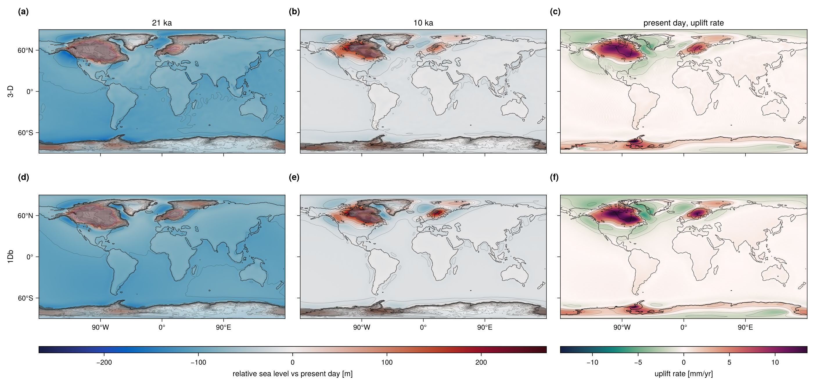
Figure 1: Relative sea level during the last deglaciation in VILMA2 with the 3-D viscosity and the toroidal field (a–c) and its radial mean, 1Db (d–f), at \(\ell_\max = 170\). (a, d) 21 ka and (b, e) 10 ka, relative to each run’s own present day; (c, f) present-day uplift rate of the bedrock. Contours show the ice surface. Model f0c4678, albedo.

The ocean-mean relative sea level at present day, relative to the reference state, is 96.84 m (3-D) and 97.06 m (1Db). This is 102.8 % and 103.2 % of the above-flotation volume of the reference ice that is lost, 94.19 m and 94.08 m in barystatic metres, both rebuilt from the run’s own output. The lateral viscosity changes relative sea level by 16.4 m RMS at 21 ka (3-D minus 1Db, at most 221 m) and the present-day uplift rate by 0.62 mm/yr RMS (at most 22.7 mm/yr).

Results

Relative sea level (RSL) is taken relative to each run’s own present day. The difference is VILMA2 minus VILMA1. All statistics are over the global grid. The difference is therefore zero at present day by construction, and present day is covered by the uplift rate instead.

Table 1: RSL difference, VILMA2 minus VILMA1, 3-D viscosity, VILMA2 with the toroidal field.

time	RMS [m]	max \|Δ\| [m]	99th pct [m]	VILMA2 signal max [m]	RMS / signal	deg 0 [m]	\|deg 1\| [m]	RMS after deg 0+1 [m]
21 ka	2.597	59.962	6.625	431.9	6.01e-03	0.12	0.30	2.607
14 ka	2.251	56.244	5.769	400.0	5.63e-03	0.24	0.25	2.247
8 ka	1.028	16.345	3.004	178.6	5.75e-03	0.13	0.15	1.021
2 ka	0.171	2.691	0.577	43.8	3.89e-03	0.02	0.03	0.169

Table 2: RSL difference, VILMA2 minus VILMA1, 1Db viscosity (radial mean of the 3-D field).

time	RMS [m]	max \|Δ\| [m]	99th pct [m]	VILMA2 signal max [m]	RMS / signal	deg 0 [m]	\|deg 1\| [m]	RMS after deg 0+1 [m]
21 ka	0.626	6.276	1.811	425.5	1.47e-03	-0.28	0.06	0.557
14 ka	0.477	4.135	1.825	379.0	1.26e-03	-0.09	0.03	0.467
8 ka	0.235	3.191	1.011	229.4	1.02e-03	-0.02	0.02	0.233
2 ka	0.045	0.703	0.181	31.6	1.42e-03	0.00	0.00	0.045

With the radial-mean viscosity the two codes agree to 0.2 % of the RSL signal throughout; the RMS difference is at most 0.66 m (24 ka). With the 3-D viscosity they agree to 0.7 % at most; the RMS difference peaks at 2.67 m (23 ka). The degree-0 and degree-1 parts of the difference stay at or below about 0.3 m in both pairs, and removing them changes the RMS by less than 0.07 m.

Table 3: Present-day uplift rate and global-mean quantities, VILMA2 against VILMA1.

quantity	3-D	1Db
Present-day uplift rate, RMS difference [mm/yr]	0.0956	0.0296
Present-day uplift rate, max difference [mm/yr]	3.1933	0.8907
Present-day uplift rate, 99th pct difference [mm/yr]	0.2961	0.0915
Present-day uplift rate, VILMA2 signal max [mm/yr]	36.78	15.54
Present-day uplift rate, RMS / signal	2.60e-03	1.91e-03
Barystatic sea level, max difference over the run [m]	0.298	0.238
Barystatic sea level, difference at present day [m]	0.292	0.232
Ocean-mean RSL at present day, VILMA2 [m]	96.84	97.06
Ocean-mean RSL at present day, VILMA1 [m]	96.55	96.83
Ocean-mean RSL at present day, difference [m]	0.29	0.23

Table 4: Grid cells on which the ocean functions of the two runs differ.

time	3-D: cells differing	3-D: % of grid	1Db: cells differing	1Db: % of grid
21 ka	4	0.002	4	0.002
14 ka	30	0.013	17	0.007
8 ka	131	0.056	52	0.022
2 ka	178	0.077	50	0.021
0 ka	210	0.090	58	0.025

For scale, the lateral-viscosity signal within VILMA2 (3-D minus 1Db: 16.4 m RMS at 21 ka, 14.4 m at 14 ka, 6.2 m at 8 ka) is about six times the difference between the codes with the 3-D viscosity, and about twenty-five times the difference with the 1Db viscosity.

Run time. With the 1Db viscosity VILMA2 runs about five times faster than VILMA1. With the 3-D viscosity VILMA2 is 11 % faster without the toroidal field and 31 % slower with it, the default (Table 5). Both solvers run behind the same driver, so forcing, diagnostics and output are included in both.

Table 5: Wall time of the 26 kyr deglaciation at \(\ell_\max = 170\), one run each with 64 threads on a shared albedo node, from the jobs’ own accounting (validation/tables/v2v1.md). Model f0c4678.

run	viscosity	wall time [min]	per kyr [min]	relative to VILMA1
VILMA2, toroidal on	3-D	69.4	2.67	1.31
VILMA2, toroidal off	3-D	47.3	1.82	0.89
VILMA1	3-D	52.9	2.03	1
VILMA2	1Db	2.8	0.11	0.21
VILMA1	1Db	13.4	0.52	1

Figures

Figure 2: VILMA2 against VILMA1 with the 3-D viscosity of Bagge et al. (2021), VILMA2 with the toroidal field. Both codes solve the same problem: the same GLAC-1D forcing, reference state, viscosity field, grid (\(\ell_\max = 170\)) and degree-1 frame. (a, d, g) VILMA2. (b, e, h) VILMA1. (c, f, i) VILMA2 minus VILMA1. The top and middle rows show relative sea level at 21 ka and 8 ka, relative to each run’s own present day. The bottom row shows the present-day uplift rate of the bedrock. The two model columns share a color scale. The difference column has its own, narrower scale. Model f0c4678, albedo.

Figure 3: VILMA2 against VILMA1 with the 1Db viscosity, the radial mean of the 3-D field. Panels as in Figure 2. Model f0c4678, albedo.

Figure 4: Size and composition of the difference in relative sea level, VILMA2 minus VILMA1, through the last deglaciation, for the 3-D viscosity (red), the 3-D viscosity with VILMA2’s toroidal field off (dark red) and the 1Db viscosity (blue), all at \(\ell_\max = 170\) on the same reference state. (a) RMS difference over the global grid. (b) The same, as a percentage of the largest absolute relative sea level that VILMA2 produces at that time. (c) The degree-0 (solid) and degree-1 (dash-dotted) parts of the difference, from an area-weighted least-squares fit. (d) Fraction of grid cells on which the ocean functions of the two runs differ. Sea level is relative to each run’s own present day, so the difference is zero at 0 ka and (b) is undefined there. Model f0c4678, albedo.

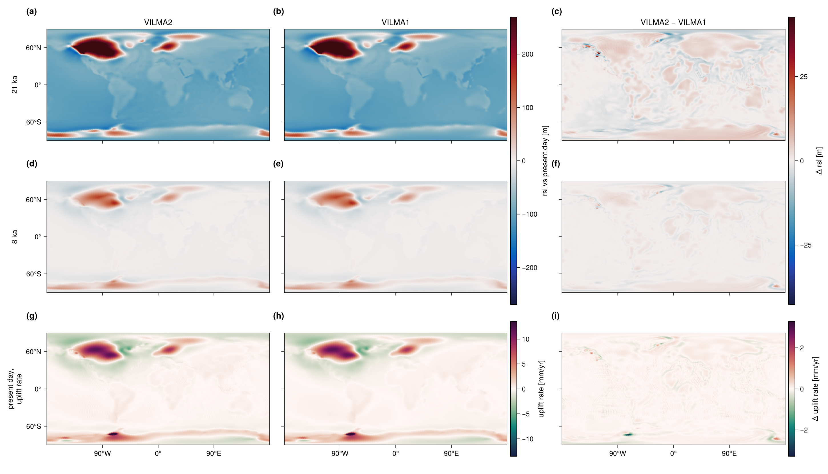
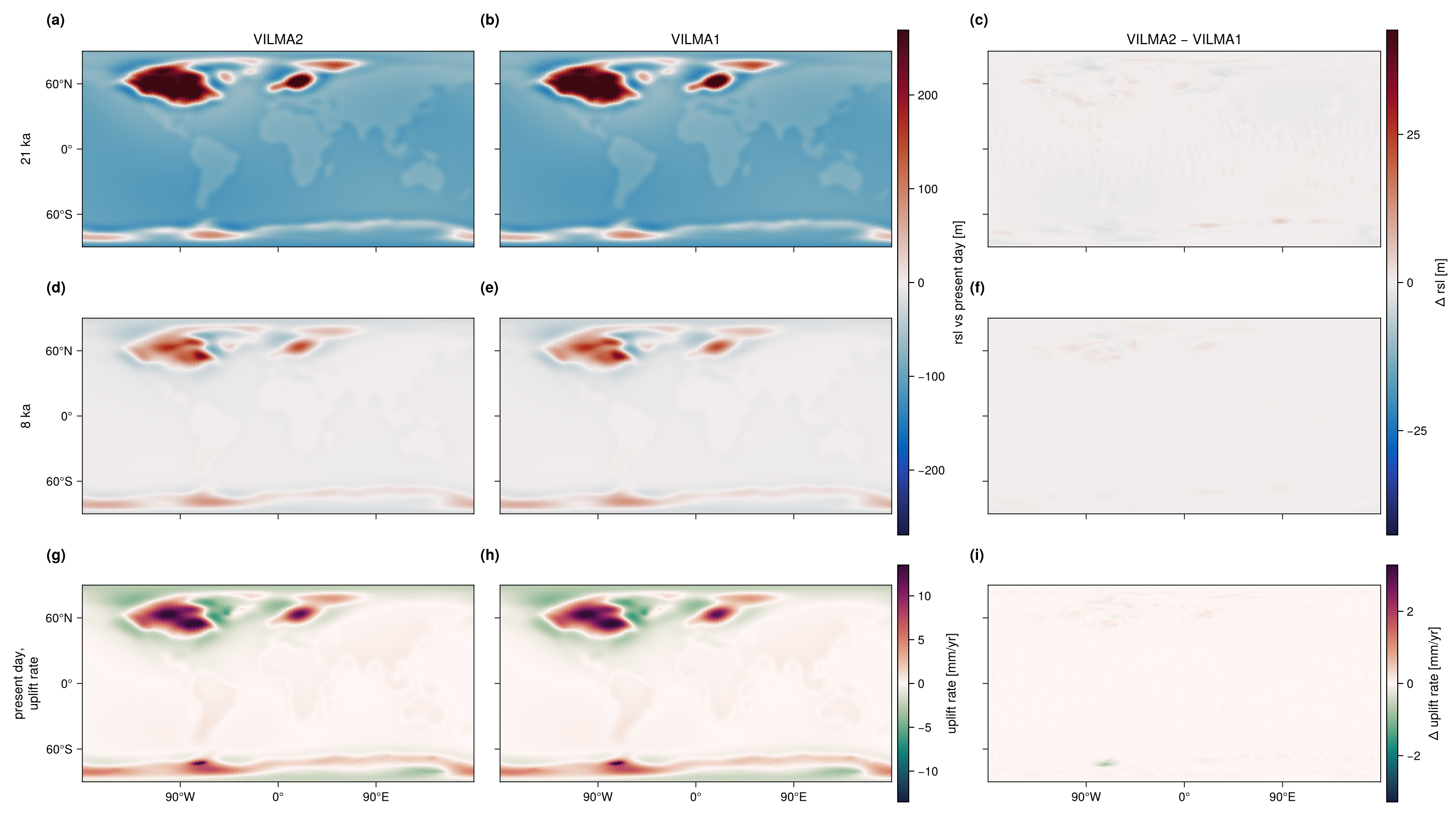
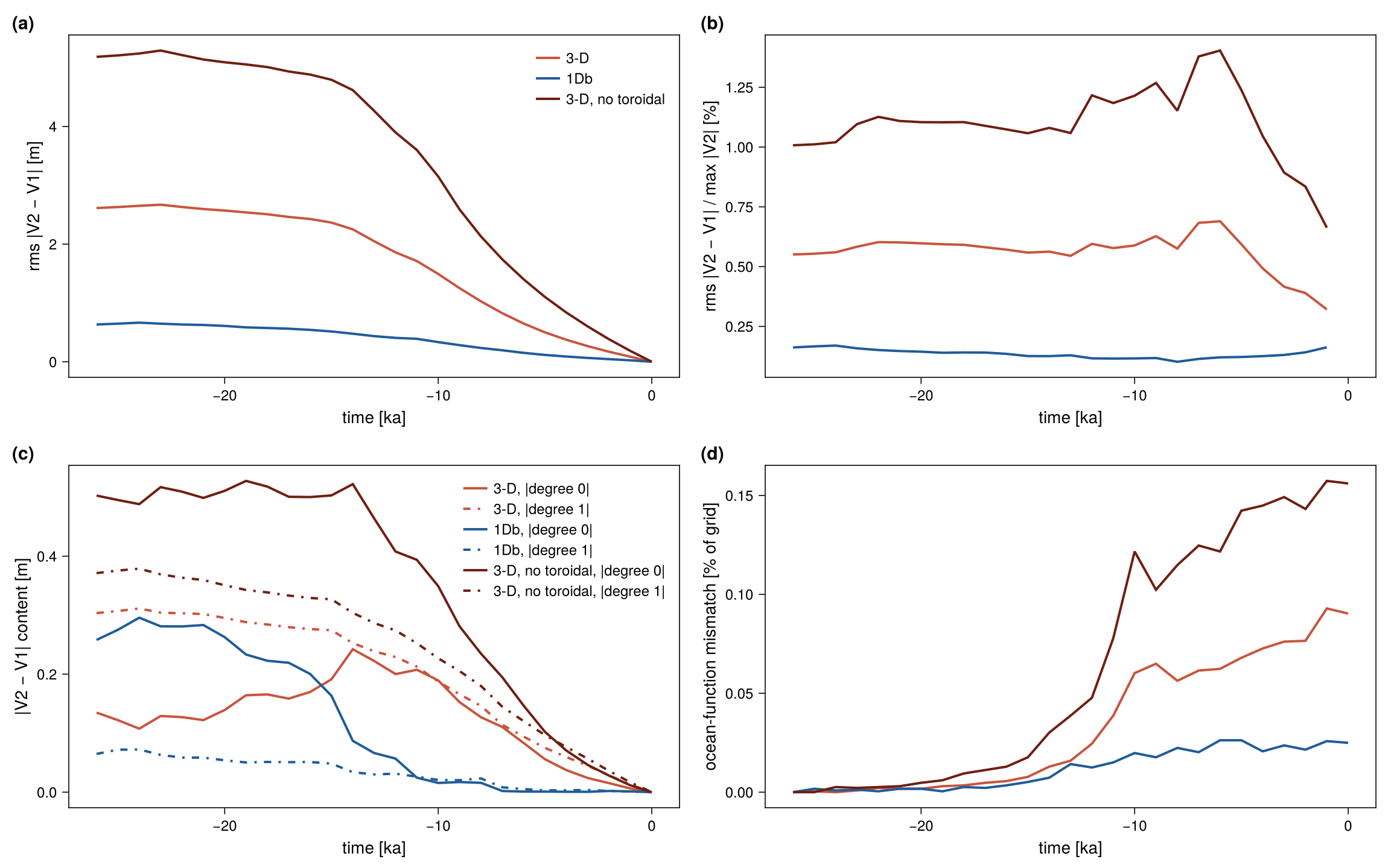
The two maps figures use a separate color scale for the difference column. On the scale of the model columns, the difference would not be visible. The summary figure shows the difference through time, and its panel (c) is the check that the degree-1 frame is matched.

Sources of difference

1. Sub-steps within a coupling interval

Both solvers reach the same load at the end of each 100 yr interval. VILMA2 ramps the load linearly across the interval and takes equal sub-steps at its own Maxwell stability limit. VILMA1 takes 12 uniform sub-steps of 8.33 yr. With 24 and 48 sub-steps, VILMA1’s result changed by 0.006 m, so the sub-step choice is not a material source of difference.

2. Radial discretisation and lateral viscosity

The two codes integrate the same viscosity field and the same elastic layer table on their own radial element grids, with the same target spacing but not the same nodes: VILMA2 spreads the elements of a layer evenly, VILMA1 truncates each layer to whole elements. With lateral variation, each code also carries it in its own way; VILMA2 treats only the elements whose lateral spread exceeds visc_3d_tol = 1e-3 as 3-D (82 of 220). The lateral variation is the only difference between the 3-D and the 1Db pair, and the 3-D pair differs about four times more (2.60 against 0.63 m RMS at 21 ka); without VILMA2’s toroidal field it would be eight times (next section). The residual of the 3-D pair is not a low-degree pattern: at 21 ka the largest single part up to degree 8 is degree 5, order 2, at 0.35 m of an area-weighted RMS of 2.18 m, so most of it lies above degree 8. The maps place it along the margins of the ice sheets and the steep viscosity gradients of the cratonic keels.

3. Toroidal field

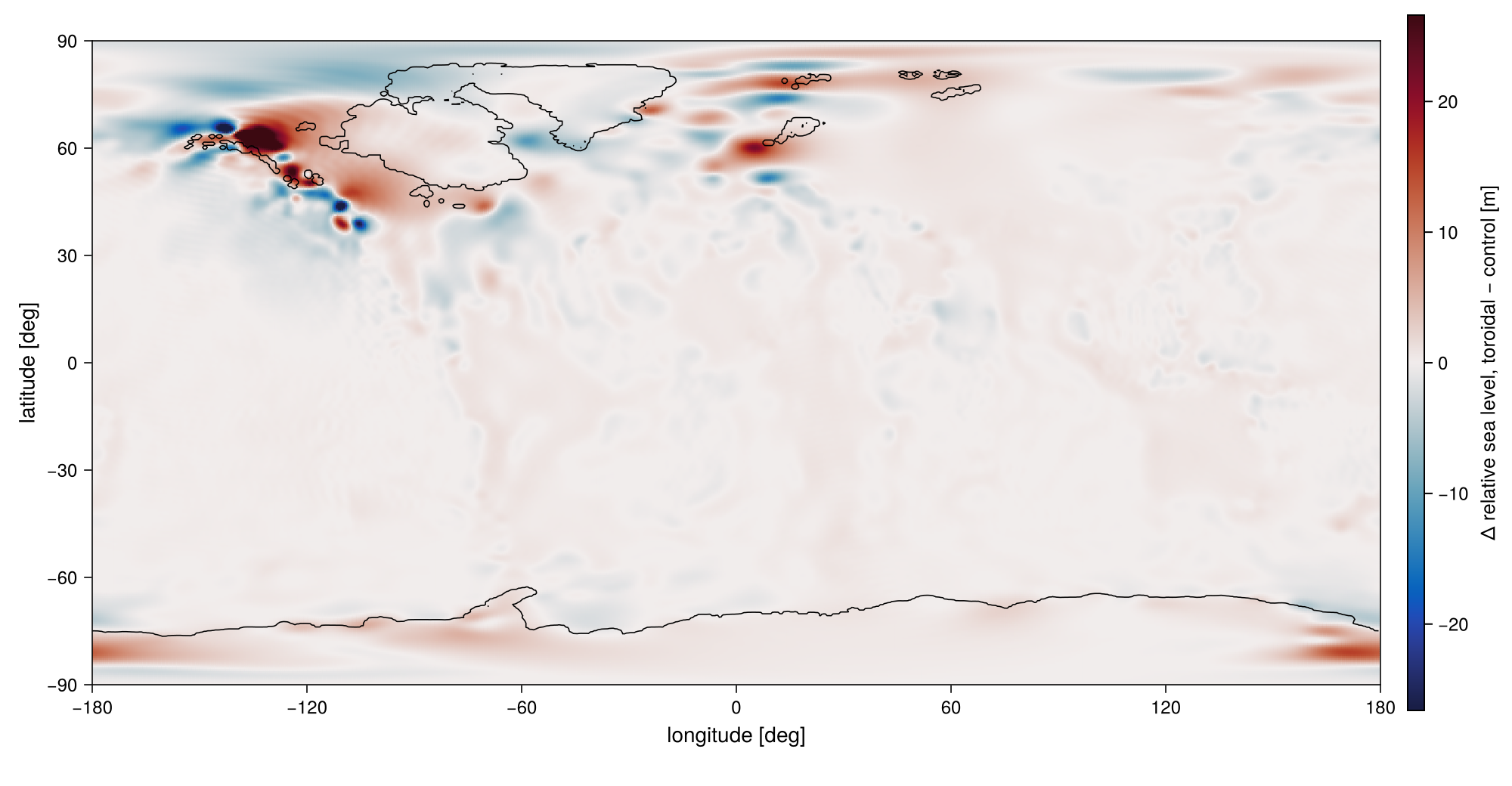
Lateral viscosity drives toroidal flow. VILMA1 includes it; VILMA2 includes it with l_toroidal = .true., the default (.false. gives a faster run without it). A control run, identical to the 3-D run but for l_toroidal = .false., measures both its effect and how much of the 3-D residual it explains (validation/tables/toroidal.md, v2v1.md).

Table 6: The 3-D run of VILMA2 with and without the toroidal field. V2 − V1 as in Table 1 (RSL relative to each run’s own present day, grid RMS).

quantity	toroidal off	toroidal on
V2 − V1 RMS of RSL at 21 ka [m]	5.14	2.60
V2 − V1 RMS of RSL at 14 ka [m]	4.62	2.25
V2 − V1 RMS of RSL at 8 ka [m]	2.13	1.03
V2 − V1 RMS of present-day uplift rate [mm/yr]	0.183	0.096
Ocean-mean RSL at present day, VILMA2 [m]	96.90	96.84
Budget closure, delivered / target [%]	102.86	102.82
Wall time per kyr of deglaciation [min] (64 threads)	1.82	2.67

Without the toroidal field, the difference between the codes doubles at every time. The field itself changes RSL, measured against the LGM reference, by 0.6 m RMS at 21 ka, 2.1 m at 10 ka and 3.0 m at present day, and by up to 92 m locally at 10 ka, around the margins of the Cordilleran, Laurentide and Fennoscandian ice sheets (Figure 5). It changes the present-day uplift rate by 0.10 mm/yr RMS and up to 2.6 mm/yr, and the ocean-mean sea level by 0.06 m. It costs a factor of 1.47 in run time.

Figure 5: Relative sea level at 10 ka, VILMA2 with the toroidal field on minus off, 3-D viscosity, \(\ell_\max = 170\), measured against the LGM reference. The color scale is clipped; the extreme is 92 m. Model f0c4678, albedo.

4. Degree-1 frame

The two codes must report RSL in the same degree-1 frame. VILMA1 works in the center-of-mass frame and carries geocenter motion in its RSL. With deg1_frame = "cm" in VILMA2 the frames are matched; panel (c) of Figure 4 shows the degree-0 and degree-1 parts of the difference stay below 0.53 m in every pair. Unmatched, degree 1 was about half of the difference in this experiment and 98 to 99.7 % of it in a disc-load test.

5. Rotational feedback (resolved)

Earlier passes (model 907bc74) were dominated by one pattern of degree 2 and order 1, the pattern of the rotational feedback. Three fixes to VILMA2’s rotation (304f4cb: the sign of the centrifugal potential, the viscosity of the relaxation, and the coupling of the rotation within the step) removed it.

Table 7: Degree-2, order-1 content of the RSL difference at 21 ka, area-weighted.

pair	RMS [m]	degree-2, order-1 part [m]	RMS after removing it [m]
3-D, now	2.18	0.49	2.12
1Db, now	0.59	0.37	0.45
3-D, 907bc74	8.91	7.74	4.41
1Db, 907bc74	7.93	7.86	1.04

VILMA1 does not write its polar motion through this driver, so the two codes are not compared on polar motion here. VILMA2’s polar motion over the run is between −2.1e-3 and 2.3e-4 (dimensionless, both components, both structures).

How to reproduce

The experiment pipeline lives in the repository’s validation/ directory. It stages the forcing, the reference state and the matched viscosity files, runs both solvers, reduces their output, and writes the tables (validation/tables/) and the figures on this page. validation/RESULTS.md records the model commit and the jobs of each pass.

cd validation
./run.sh build              # model, benchmark drivers, VILMA1-backend binary
./run.sh ref                # LGM reference state
./run.sh submit prep        # export the reference, write the shared viscosity files
./run.sh D V1 T             # VILMA2 (3-D toroidal off, 1Db), VILMA1, VILMA2 3-D toroidal on
./run.sh submit reduce analyse

The VILMA1 runs need a build with vilma_v1=1 and a VILMA1 install. VILMA1 is a precompiled library and is not a dependency of the default build. The build, the namelist keys and the constraints are described in doc/vilma-v1-backend.md. examples/deglac_vilma_v1.nml is a low-resolution template for the backend. It is not the configuration of this page.

References

Bagge, M., V. Klemann, B. Steinberger, M. Latinović, and M. Thomas. 2021. “Glacial-Isostatic Adjustment Models Using Geodynamically Constrained 3D Earth Structures.” Geochemistry, Geophysics, Geosystems 22 (11): e2021GC009853. https://doi.org/10.1029/2021GC009853.

Martinec, Z. 2000. “Spectral–Finite Element Approach to Three-Dimensional Viscoelastic Relaxation in a Spherical Earth.” Geophysical Journal International 142 (1): 117–41. https://doi.org/10.1046/j.1365-246x.2000.00138.x.

Martinec, Z., V. Klemann, W. van der Wal, et al. 2018. “A Benchmark Study of Numerical Implementations of the Sea Level Equation in GIA Modelling.” Geophysical Journal International 215 (1): 389–414. https://doi.org/10.1093/gji/ggy280.