greenland
3D offline benchmark — test_greenland.x
What it tests
test_greenland.x runs elsa on a real ice sheet: the Greenland domain at 16 km, forced offline from a Yelmo restart (data/initmip-grl-16km/yelmo_restart.nc, the same file that the tracer package uses, so that the two schemes can be compared on identical host fields).
The restart carries no spun-up isochrone field, so there is no known answer against which to compare. This is therefore a structural check — against a real velocity field, real staggering, real non-uniform sigma levels and a real ice margin — rather than a comparison with a closed-form solution.
Source: src/test_greenland.f90. Run it with make run-greenland; it writes output/GRL-16KM/elsa.nc.
Staggering in practice
Yelmo writes ux/uy on staggered acx/acy nodes. elsa’s advection requires face velocities — which is exactly what acx/acy nodes are — so they are handed over as-is with stagger = "acx_acy", and nothing is destaggered. The tracer package reads the same file and does destagger to cell centres, since it requires cell-centred velocities. This contrast is the motivation for expressing staggering as a coordinate rather than as a conversion.
What is checked
At every update, on both a native (grid_factor = 1) and a coarsened (grid_factor = 2.5) run:
- layer thicknesses remain finite and non-negative;
- every column sums to the host’s ice thickness (closure error 0 at
grid_factor = 1, and around \(10^{-15}\) coarsened); - ice-free columns carry no layers;
- isochrones remain ordered — younger ice sits higher, and none escapes the ice column;
- at
grid_factor = 1, the conservative map reproduces the host ice thickness exactly, and volume is conserved; - reseeding of emptied margin columns remains rare (a handful of thin cells per step, out of around 7000).
The output
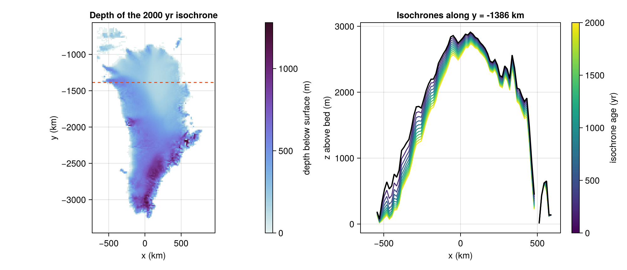
Restart is bit-identical
The benchmark also runs the restart round-trip: a continuous run, and the same run stopped halfway, written to a restart file, and picked up again. The two runs end with
\[ \max_{i,j,k}\bigl|\,d^{\text{restart}}_{ijk} - d^{\text{continuous}}_{ijk}\,\bigr| = 0. \]
Bit-identical, and not merely close. This is the only check strong enough to catch a piece of state — n_top, the isochrone schedule, the previous-step ice thickness — being reconstructed rather than carried. See Design for what the restart stores and why d_iso must be written in double precision.
Performance
At 16 km (19 186 cells and 20 layers), a 2000-year run spends 0.38 s in elsa_update on one core, and 0.15 s on eight. The cost is linear in simulated time and in layer count, and the total sub-step count does not depend on the coupling period. Extrapolating to the Rieckh et al. (2024) control configuration — 160 kyr, and around 415 layers on average — gives a run time on the order of 20 minutes on a single core, against the roughly 24 h of ELSA time implied by that paper’s Fig. 9. The machines differ, so this should be treated as an order-of-magnitude comparison.